In 2020 as a result of lockdown I was asked to help create a course for MRes students as an introduction to computer-aided drug design [DOI] that they all complete at home.

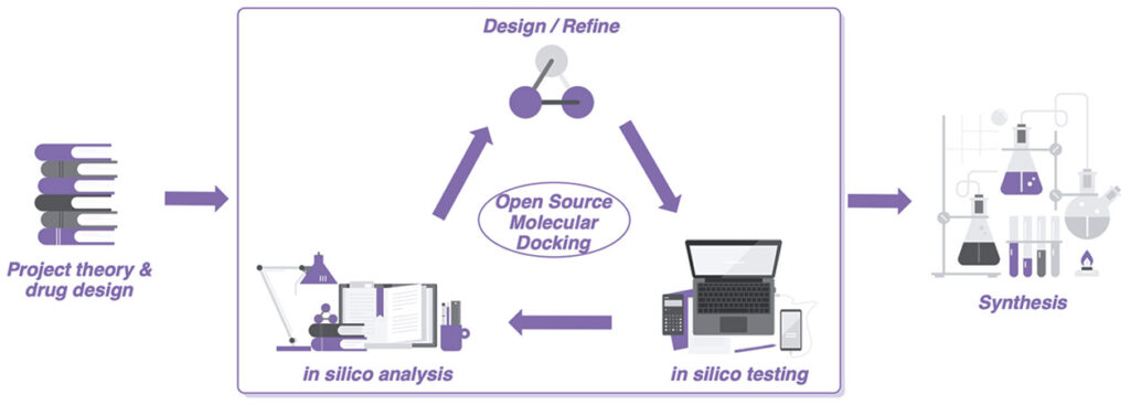
This work lead to the above publication which has had over 18,500 total views and been downloaded almost 5000 times.

There is also a lab manual and the old Jupyter notebook all of which are freely available on GitHub

https://github.com/UCL/Open_Docking_Lab_Handbook

Over the years I’ve updated the notebook to fix bugs and add features that students at different universities have requested, the result is a project that become a little unwieldy and I thought I’d spend a few weeks (with Claude) cleaning it all up and making it a lot more efficient.

This notebook does not include the preparation of the target protein for docking, but here are a few of the things that need to be addressed.

–Alternates, Residues with alternate locations and/or ambiguous sequence identities (choose highest occupancy) but remember proteins are not static.

–Termini, Protein chain C- or N-termini which need to be charged or capped, or if DNA the terminal PO4 may only have three oxygens bonded to the phosphorous and an additional oxygen needs to be added. Sometimes loops are very disordered and appear as a breaks in the chain, it may be possible to use a loop library to model a replacement.

–Hydrogens, usually not visible and so need to be added/checked, particularly check hydrogens on heteroatoms, especially active site residues where the local environment may influence pKa

–Ligand, Novel ligands in particular need checking to confirm atoms and bond orders are correct (PDB files do not contain bond information)

–Conformation, check that torsions are reasonable and there are no clashes.

–Charge, It with worth checking the charge on all ionisable groups.

–It can be difficult to be certain of the position of nitrogens in His or the primary amide in Asn, Gln.

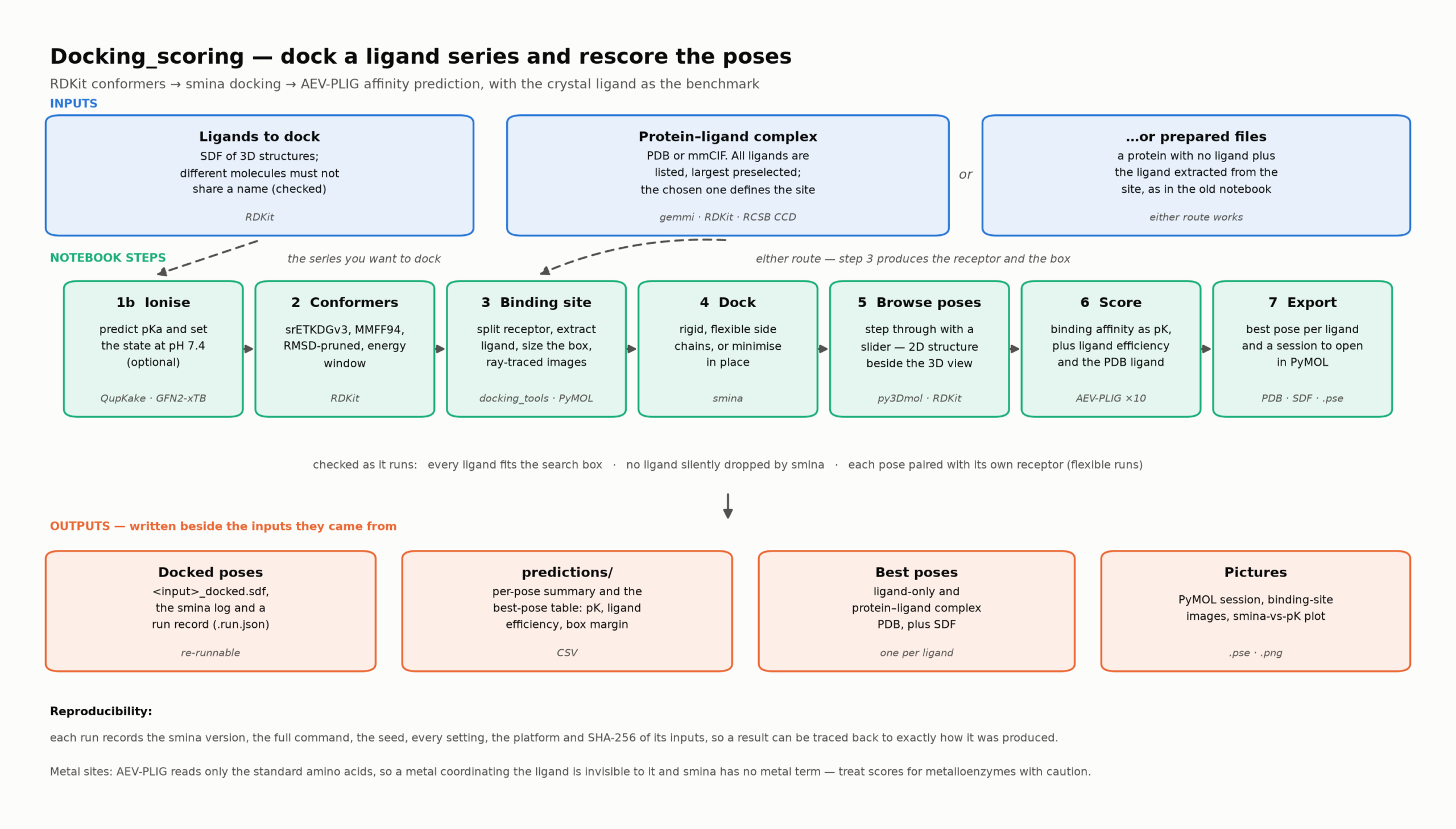
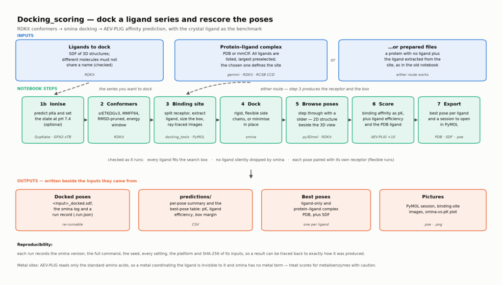
The new README for the docking and scoring is shown below

Docking_scoring

A Jupyter notebook for docking ligands into a protein with smina and rescoring the poses with the AEV-PLIG binding-affinity model. It covers conformer generation, binding-site preparation, rigid or flexible docking, pose viewing, affinity prediction using AEV-plig and export in a variety of formats.

The example is the SARS-CoV-2 main protease (Mpro) fragment structure 5RHD. A fully run copy of the notebook is in DockingScoring.html (download it and open it in a browser to see the outputs and interactive 3D views) and, for printing or quick viewing on GitHub, DockingScoring.pdf.

Workflow

Ligands. Load an SDF of 3D structures, check that the names are unique, and browse the molecules with a slider.
1b. Ionisation states. Optionally predict each ligand’s ionisation state at a chosen pH with QupKake (micro-pKa prediction), and dock the ligands in those states.
Conformers. Generate conformers with RDKit srETKDGv3 (or ETKDGv3, ETKDG, ETDG), pruned by RMSD, MMFF94-minimised and filtered by an energy window. Undefined stereocentres can optionally be enumerated.
Binding site. Either:
- load a protein–ligand complex PDB and pick the ligand that defines the site, or
- supply prepared files: a protein without the ligand plus the extracted ligand.
Images. Ray-traced PyMOL images of the whole protein with the ligand bound, and of the ligand in the binding site.
Docking. An smina input panel for rigid docking, flexible side chains, or --minimize.
Results. Step through the poses in 3D with a slider.
AEV-PLIG. Predict the pK of every pose, and score the ligand from the PDB in its crystal pose as a reference.
Export. Write the best pose of each ligand as PDB files and as a PyMOL session.

Setup

Run these commands from the repository folder.

1. Conda environment and Jupyter kernel

conda env create -f environment.yml

conda run -n docking_scoring python -m ipykernel install --user --name docking_scoring --display-name "Python (docking_scoring)"

environment.yml is portable (macOS and Linux) and installs current versions. docking_scoring.yml pins the exact versions this was developed and tested with on an Apple-silicon Mac. It has never been tested under Windows and the best option might be to try Windows Subsystem for Linux .

Package	Tested version
Python	3.12
RDKit	2026.09
PyTorch	2.10 (conda-forge)
torch-geometric	2.8
torchani	2.9
PyMOL (open source)	3.1
Open Babel	3.2
gemmi	0.7
py3Dmol	2.5
ipywidgets	8.1
JupyterLab	4.6

Install PyTorch from conda-forge, not pip. The pip wheel bundles its own OpenMP library, which clashes with conda’s and crashes on import with OMP: Error #15.

2. AEV-PLIG trained models

The trained models (about 300 MB) are not stored in this repository. Download them from the official AEV-PLIG repository:

conda run -n docking_scoring python aev_plig/download_models.py

The script fetches the 10-model model_GATv2Net_ligsim90_fep_benchmark ensemble and its scaler from a fixed upstream commit, checks each file’s checksum, and saves them to aev_plig/output/trained_models/.

3. smina

smina is not included in environment.yml: the conda-forge smina package (2020 build) needs an old version of Boost that forces an old RDKit. Install it in one of two ways:

A separate conda environment, which the notebook finds automatically: conda create -n smina -c conda-forge smina
The prebuilt binary from https://sourceforge.net/projects/smina/. Make it executable (chmod +x), then put it on your PATH or set the SMINA environment variable to its full path.

The notebook looks for smina in this order:

the SMINA environment variable;
smina, smina.static or smina.osx.12 in the notebook’s environment or on the PATH;
a conda environment called smina;
/usr/local/smina.osx.12 and other common locations.

You can also type the path into the smina panel.

4. Run

Open DockingScoring.ipynb in JupyterLab with the Python (docking_scoring) kernel.

Each step has a panel with a Run or Apply button. Running all cells sets the panels up but does not start the long jobs.
To run every step with the default settings, set AUTO_RUN = True in the first code cell.

Project layout

DockingScoring.ipynb         the notebook
DockingScoring.html          a fully run copy of the notebook (static)
DockingScoring.pdf           the same, as a PDF (A4 landscape)
docking_tools.py             all helper code (panels, viewers, docking, scoring, export)
environment.yml              conda environment (portable)
docking_scoring.yml          exact tested environment (macOS arm64)
aev_plig/                    AEV-PLIG prediction code (models: aev_plig/download_models.py)
example/                     5RHD example inputs; results are written here when you run the notebook

Generated results are not tracked in git (see .gitignore). Run the notebook to recreate them, or see DockingScoring.html.

Inputs

Ligand SDF

3D structures, ideally with hydrogens.
Each record needs a name on its first line.
smina keeps only that name, and the results are grouped by it, so different structures must not share a name.

The notebook checks for duplicate names. If it finds any, it offers two fixes:

use an SD field with a unique value for every molecule (e.g. ID, IDNUMBER, Record_ID) as the ligand ID, or
assign unique names automatically (name, name_2, …).

The original name is kept in the original_name property, and the input file is not modified.

Binding site

Complex structure mode (PDB or mmCIF)

Reads .pdb and mmCIF (.cif, .mmcif, optionally gzipped). mmCIF is the PDB’s standard format, and is read with gemmi.
Lists all ligands, with chemical names where the file has them, and selects the largest automatically. The panel says which one was chosen; pick another from the list if the file holds several ligands.
Hides waters, solvents and crystallisation additives (e.g. DMSO, glycerol, PEG, sulfate), ions, and terminal caps such as NME. Tick Also list solvents, ions, additives and caps to show them.
Uses only the first alternate location (A) of the protein and ligand.
Bond orders for the extracted ligand come from, in order of preference:
1. a SMILES template, if you paste one. Its charges are kept, so it can set the protonation state;
2. the ligand’s hydrogens and formal charges (RDKit), when hydrogens are present;
3. the ligand’s entry in the PDB Chemical Component Dictionary, fetched from RCSB, for files without hydrogens such as RCSB X-ray structures. It is used only if its heavy atoms match, and gives the neutral molecule;
4. Open Babel perception from the geometry.
The protein file keeps the HELIX and SHEET records, but other HET groups and waters are removed. Metal ions are kept unless you untick that option.
Output files are named after the input, e.g. 5RHD_protein.pdb. mmCIF input adds _cif (5RHD_cif_protein.pdb), so it never overwrites files made from a PDB file of the same entry, which may use a different coordinate frame.

Example: example/5RHD.pdb was prepared in MOE (hydrogens added, piperazine protonated, ligand named LIG). example/5RHD.cif is the RCSB file: its ligand US7 has no hydrogens and is taken as the neutral molecule. Paste CS(=O)(=O)c1ccc(N2CC[NH2+]CC2)cc1 as the SMILES template for the protonated form. Using the CIF gave the same best-pose AEV-PLIG pK for FromXRay (5.31) as the PDB file.

Prepared-files mode uses your protein and ligand PDB files as they are.

Note: The two modes can give different smina scores for the same ligand. For example, proteinNoligand.pdb keeps the waters and DMS molecules, which add contacts. Compare runs that used the same mode.

Outputs

Docked poses are stored as SDF files. The best pose of each ligand is also exported as PDB files (ligand only, and protein–ligand complex) and as a PyMOL session file.

Every output is written next to the input it was derived from.

File	Location
`<input>_pH7.4.sdf` / `.csv` (ligands in QupKake-predicted ionisation states) and `qupkake/`	next to the ligand SDF
`<input>_confs.sdf`	next to the ligand SDF
`<stem>_protein.pdb`, `<stem>_ligand_<RES><chain><num>.pdb/.sdf`	next to the complex PDB
`<stem>_complex.png`, `<stem>_site.png`	next to the binding-site input
`<input>_docked.sdf` / `_flexdocked.sdf` / `_minimized.sdf`, plus `.log` and `.run.json` (run record)	next to the ligand SDF
`<output>_flexres.pdb` (flexible docking: one model per pose)	next to the docked SDF

All prediction results go to a predictions/ folder next to the docked SDF:

File	Contents
`<docked>_summary.csv`	every pose: smina score, AEV-PLIG pK (10-model mean ± std), heavy atoms, ligand efficiency, box margin, best-pose flags
`<docked>_run_info.json`	run record: docking and scoring settings, software versions, input checksums
`<docked>_best_poses_table.csv`	best pose per ligand, plus the PDB ligand row (AEV-PLIG pK, smina scores, ligand efficiency, box margin)
`<docked>_scored.sdf`, `<docked>_best_poses.sdf`	poses annotated with pK
`best_poses_pdb/<docked>/`	best pose per ligand as `_ligand.pdb` and `_complex.pdb` (ligand = chain L, resname LIG)
`<docked>_best_poses.pse`	PyMOL session of the best poses
`<docked>_smina_vs_aevplig.png`	smina score vs pK; the dashed line is the PDB ligand
`poses/<docked>/`	per-pose AEV-PLIG inputs (and per-pose receptors after flexible docking)
`pdb_ligand/`	the PDB ligand as scored by smina, its minimised pose and the log
`<docked>_aevplig_input.csv`, `<docked>_predictions.csv`, logs	raw AEV-PLIG input and output

Copies of the docked SDF, receptor, reference ligand, conformers and images are also placed in predictions/, so the folder is a self-contained record.

Search box

smina docks only inside the search box: the extent of the autobox ligand (all atoms, hydrogens included) plus autobox_add (default 4 Å) on every side. Atoms outside the box are heavily penalised during the search, and smina gives no warning when a ligand is too large. The ligand is simply squeezed: it curls up, or groups that would reach a neighbouring sub-pocket point elsewhere.

Before docking, the smina panel shows the box size and compares each ligand’s longest heavy-atom span, taken from the conformer file, with the smallest box side:

Status	Meaning
ok	at least 2 Å to spare
tight	less than 2 Å to spare
longer than smallest box side	the ligand can only fit along a diagonal

When any ligand is tight or longer, the panel suggests an autobox_add. It also warns above Vina’s recommended 27,000 Å³.

After docking, smina’s output reports how many poses have a heavy atom within 1 Å of a box face. The summary and best-poses tables add box_margin, the closest heavy-atom distance to a face in Å (negative means outside), and at_box_edge. A best pose at the box edge means the box may have limited that ligand: re-dock with a larger autobox_add, or set the box explicitly with --center_x/y/z --size_x/y/z under “extra arguments”.

Example (5RHD fragment + 4 Å = 16.8 × 13.2 × 15.5 Å):

Phenyl (11.4 Å) and iProAmine (11.9 Å) are tight.
38 of 297 poses come within 1 Å of the edge, and 3 have an atom slightly outside.
iProAmine’s best AEV-PLIG pose is 0.13 Å outside the box.

The box is stored in each run record (<output>.run.json).

Ligand efficiency

The summary and best-poses tables include ligand efficiency (LE), the binding free energy per heavy atom, in kcal/mol per heavy atom:

Column	Definition
`heavy_atoms`	number of non-hydrogen atoms
`LE_AEV_PLIG`	1.364 × pK / heavy atoms, from the AEV-PLIG pK (ΔG = −2.303 RT pK at 298 K)
`LE_smina`	−(smina score) / heavy atoms

An LE of about 0.3 or more is the usual guide for a good starting point. Small fragments such as the 5RHD series (15–21 heavy atoms) typically score 0.4–0.5 on LE_AEV_PLIG.

Note: After flexible docking, LE_smina is inflated, because the flexible smina score appears to include the flexed side chains. Use LE_AEV_PLIG to compare across docking modes.

Ionisation states (QupKake)

QupKake (Abarbanel & Hutchison, J. Chem. Theory Comput. 2024, https://doi.org/10.1021/acs.jctc.4c00328) predicts micro-pKa values from GFN2-xTB calculations and graph neural networks. Step 1b of the notebook uses it to set the ionisation state of the input ligands and of the ligand from the PDB.

How the state is set:

Each ligand is neutralised and submitted to QupKake, which predicts a pKa for every basic and acidic site.
At the chosen pH (default 7.4), the most basic site is protonated if its pKa is above the pH, and the most acidic site is deprotonated if its pKa is below it. At most one of each is applied. Other sites that also cross the pH are reported, not applied.
Implausible basic sites are ignored (on by default; untick the box to use every site). For this ligand series QupKake reported sulphonamide N, amide N and aryl-amine N, such as the N-aryl nitrogen of an aryl-piperazine, as the most basic sites. Taken at face value, that would protonate a sulphonamide ([NH3+]S(=O)(=O)…).

The ligands in their predicted states are written to <input>_pH7.4.sdf, with a table in <input>_pH7.4.csv. When docking in the predicted states is ticked, that file is docked, so every later output is named <input>_pH7.4_… and never overwrites the results for the input states. The PDB ligand keeps its crystal coordinates and is used as the reference in the final table. QupKake’s own files are in qupkake/ next to the input.

Example result (pH 7.4). With the filter on, QupKake’s states match the MOE-prepared input exactly: the piperazine or piperidine NH is protonated, or the N-isopropyl N for iProAmine. Re-docking therefore reproduced all 297 poses and scores. The neutral US7 from 5RHD.cif is protonated to the same state.

With the filter off, 6 of the 7 ligands were charged on a sulphonamide or aryl-amine N, and the best-pose AEV-PLIG pK changed by −0.27 to +0.35:

Ligand	pK, input / QupKake (filtered)	pK, QupKake raw	Raw protonation site
iProAmine	6.87	6.77	sulphonamide NH₂
sulphonamide	6.57	6.46	sulphonamide NH₂
Phenyl	5.67	5.47	aryl N
piperidine	5.45	5.45	piperidine NH (same)
FromXRay	5.31	5.04	aryl N
DimethylN	5.22	5.57	sulphonamide N(CH₃)₂
amide	4.67	4.40	aryl N

Installing QupKake. It needs its own conda environment, named qupkake, with xtb 6.4.1 built from source; see the QupKake README. On Apple silicon, build xtb at -O2, because gfortran 16 at -O3 miscompiles it. The notebook finds the environment automatically and limits each xtb process to one thread. If QupKake is not installed, the input ionisation states are used.

Full details for installing QupKake are available here https://github.com/drc007/qupkake-apple-silicon/tree/main/qupkake-apple-silicon

Reproducibility

Every smina run writes a run record next to its output, <output>.run.json, and the same summary at the top of <output>.log. The record holds:

the smina version and path, and the full command;
seed, --cpu, exhaustiveness and every other setting;
the platform;
SHA-256 checksums of the receptor, ligand and autobox files and of the output.

AEV-PLIG adds predictions/<docked>_run_info.json, which contains that docking record plus the model, scoring options, library versions, receptor checksum and the PDB-ligand scores.

Seed and thread count. With the tested smina build (master:dc3dfab, based on AutoDock Vina 1.1.2), a fixed --seed gave identical poses whatever the --cpu value:

Mode	`--cpu` values compared	Coordinates	Reported scores
Rigid	1, 4, 8, 24	identical	identical
Flexible	1, 3, 24	identical	identical at `--cpu` 1 and 24

At --cpu 3 (fewer threads than exhaustiveness runs), flexible docking showed a run-to-run jitter of up to 0.002 kcal/mol in the reported score. That is below the 0.01 kcal/mol precision of smina’s log.

--cpu therefore defaults to the number of cores. Results can still differ with a different smina or Vina build, platform or compiler, so keep the run record with your results.

Flexible docking

Choose Flexible side chains in the smina panel.
Automatic selection takes every residue within a set distance of the ligand (default 5 Å).
Manual selection lets you pick residues from a list, or type them (A:41,A:145).
Gly, Ala and Pro are excluded, because their side chains have no rotatable bonds.

It is much slower than rigid docking. For the example’s 33 conformers:

rigid docking took about 40 s;
flexible docking with 4 residues at exhaustiveness 8 took about 8½ min.

The automatic 5 Å selection picks 13 residues for 5RHD, which would be far slower again.

smina writes the flexed side chains for every pose. They come out in the same order as the poses, but without PDB atom names. The notebook maps them back onto the receptor and rebuilds a complete receptor for each pose, which is used:

in the 3D viewer, where the flexed side chains are magenta and the original ones grey;
by AEV-PLIG, which scores each pose against its own receptor;
in the PDB and PyMOL exports.

Pairing poses with their side chains is verified, not assumed. smina writes each ligand’s poses and side-chain models together, so if it skips a ligand both files lose it and stay in step (tested). Before anything is paired, the notebook checks:

Names: the docked SDF’s record titles and the models’ names must match. If they don’t, ligand blocks are aligned by name, and a block is paired only when its pose and model counts agree.
Geometry: a pose that overlaps its own flexed side chains (< 1.5 Å) is rejected.

AEV-PLIG stops with an error on any mismatch, rather than score a pose against the wrong receptor. The viewer shows such poses with the rigid protein and a warning.

Note: The flexible-docking smina score appears to include the flexed side chains, so its values (around −8 to −11 kcal/mol for the example) are not comparable with rigid scores or with the PDB-ligand row. AEV-PLIG pK values are comparable between modes.

AEV-PLIG

aev_plig/ contains the AEV-PLIG prediction code (process_and_predict.py and its modules) from https://github.com/oxpig/AEV-PLIG, licensed under the BSD 3-Clause licence in aev_plig/LICENSE.txt. The trained model_GATv2Net_ligsim90_fep_benchmark ensemble (10 models) is downloaded separately (see Setup).

Changes for the current library versions:

torchani 2.9 changed its SpeciesConverter, so the species index is now computed directly as atomic number − 1 (equivalent).
pkg_resources is replaced by importlib.metadata.
Model weights are loaded with torch.load(..., weights_only=False), which torch ≥ 2.6 requires.
A new --output_dir option controls where the predictions are written.
Dataset paths are handled with os.path.splitext.
RDKit’s deprecated GetExplicitValence() is replaced.

Regression check: on AEV-PLIG’s example dataset, all 241 predictions from the patched code in the new environment match the original code in a Python 3.8 / torch 2.4 environment to within 2×10⁻⁶.

Hydrogens

Before scoring, all hydrogens are added to each ligand pose, because AEV-PLIG was trained on fully protonated ligands and one of its atom features counts attached hydrogens. smina writes polar hydrogens only. Scoring the same poses with every hydrogen removed changes the predicted pK by up to about 1 unit.

Citation

Valsson et al., “Narrowing the gap between machine learning scoring functions and free energy perturbation using augmented data”, Communications Chemistry (2025), https://doi.org/10.1038/s42004-025-01428-y. The licence is in aev_plig/LICENSE.txt.

Display options

Protein colouring uses the RasMol secondary-structure scheme by default: helix magenta-red, sheet yellow, coil and turn white. Coil is drawn light grey so it shows on a white background.
- Set dt.PROTEIN_COLOURING to "rainbow" or "grey" for other schemes.
- Set dt.RASMOL_COIL = "#FFFFFF" for strict RasMol white coil.
Pose viewers have toggles for the binding-site residues, the ligand from the PDB, and (after flexible docking) the original side chains.
Binding-site image has a toggle to hide the side chains.

Known limitations

smina silently stops at an unreadable SDF record. Every later ligand is skipped, the exit code is still 0, and the log says nothing. The smina panel warns before docking if the ligand file has unreadable records. After docking it compares the input ligands with the docked ones, reports any ligand with no poses, and records them in the run record (ligands_missing).
Running the notebook from the command line with jupyter nbconvert --execute stalls on the slider cells; this is an nbclient issue. All the steps still complete and their files are written. Use JupyterLab interactively.
Turns are coloured as coil unless the PDB file has TURN records, because neither 3Dmol.js nor PyMOL assigns turns.
AEV-PLIG accepts only the elements C, N, O, S, P, F, Cl, Br, I and B. Ligands with any other element are skipped, and the notebook reports how many were rejected.

Licence

The notebook, docking_tools.py and documentation are released under the MIT licence (see LICENSE) and are available on GitHub https://github.com/drc007/docking_scoring.

The bundled AEV-PLIG code in aev_plig/ keeps its own BSD 3-Clause licence (see aev_plig/LICENSE.txt). The 5RHD structure comes from the Protein Data Bank (https://www.rcsb.org/structure/5RHD).