TabPFN on Apple Silicon – Macs in Chemistry

A recent paper published in Nature caught my eye, Accurate predictions on small data with a tabular foundation model by Hollmann et al.,

Here we present the Tabular Prior-data Fitted Network (TabPFN), a tabular foundation model that outperforms all previous methods on datasets with up to 10,000 samples by a wide margin, using substantially less training time.

This foundation model was trained on around 130,000,000 synthetically generated datasets that mimic “real world” tabular data. These datasets sampled dataset size and number of features, both classification and regression tasks, and Gaussian noise was added to mimic real-world complexities.

They report TabPFN excels in handling small- to medium-sized datasets with up to 10,000 samples and 500 features, this is actually ideal for many projects. Indeed, whilst there is a huge amount of interest in very, very large global models in many cases a smaller local model performs as well or better DOI.

There is a very nice exploration of TabPFN in a cheminformatics setting here TabPFN for chemical datasets that uses the Therapeutic data commons (TDC) and RDKit descriptors. They also provide the python script used. This was used with minor modifications to allow selection of gpu or cpu, and selection of particular datasets. some datasets failed on first pass and the input data needed to be cleaned.

To install

git clone https://github.com/jonswain/tabpfn-tdc.git 
cd tabpfn-tdc
conda env create -f environment.yml
conda activate tabpfn-tdc

git clone https://github.com/jonswain/tabpfn-tdc.git

cd tabpfn-tdc

conda env create -f environment.yml

conda activate tabpfn-tdc

This creates a folder called tabpfn-tdc that contains all the data and submission python script that can be invoked with.

python submission.py | 2>&1 | tee -a log.tx

1	python submission.py \| 2>&1 \| tee -a log.tx

The python script

from time import time

import pandas as pd
import torch
from rdkit import Chem
from rdkit.Chem import Descriptors
from tabpfn import TabPFNClassifier, TabPFNRegressor
from tdc.benchmark_group import admet_group
from tqdm import tqdm


def calculateDescriptors(mol: Chem.Mol, missingVal: float | None = 0.0) -> dict:
    """Calculate the full list of descriptors for a molecule."""
    res = {}
    for nm, fn in Descriptors._descList:
        try:
            val = fn(mol)
        except: 
            val = missingVal
        res[nm] = val
    return res


def createDescriptorDataFrame(
    smiles: list[str],
    max_value: float = torch.finfo(torch.half).max,
) -> pd.DataFrame:
    """Create a DataFrame of descriptors for a list of SMILES strings."""
    mols = [Chem.MolFromSmiles(smi) for smi in smiles]
    descs = [calculateDescriptors(mol) for mol in mols]
    return pd.DataFrame(descs).clip(-max_value, max_value)


def getDeviceType() -> str:
    """Get the device type to use for training and inference."""
    if torch.cuda.is_available():
        return "cuda"
    elif torch.backends.mps.is_available(): #comment out to use cpu
        return "mps" #comment out to use cpu
    else:
        return "cpu"


def main():
    """Train and evaluate the model on the benchmark datasets."""
    # Get the device type to use for training and inference
    device_type = getDeviceType()
    print(f"Training and inference completed using: {device_type}")

    # Load the benchmark datasets
    group = admet_group(path="data/")
    predictions_list = [{}, {}, {}, {}, {}]

    for dataset_name in group.dataset_names:
        print(f"Dataset: {dataset_name}")
        start = time()
        benchmark = group.get(dataset_name)
        train_val, test = benchmark["train_val"], benchmark["test"]

        # Edit to select particular groups of datasets
        if len(train_val) > 1800:
            print(f"Skipping {dataset_name} due to size")
            continue
		
        if dataset_name != "lipophilicity_astrazeneca":
            print(f"Skipping {dataset_name} wrong name")
            continue
		
        X_train = createDescriptorDataFrame(train_val["Drug"])
        y_train = train_val["Y"]
        X_test = createDescriptorDataFrame(test["Drug"])
        y_test = test["Y"]

        print(f"Train: {X_train.shape}, {y_train.shape}")
        print(f"Test: {X_test.shape}, {y_test.shape}")

        for seed in tqdm([1, 2, 3, 4, 5]):
            params = {
                "random_state": seed,
                "n_jobs": -1,
                "n_estimators": 4,
                "device": device_type,
            }
            # TODO: Work out how to use memory saving with MPS
            if device_type == "mps":
                params["memory_saving_mode"] = True
                params["ignore_pretraining_limits"] = True

            # TabPFN has a maximum number of samples it can handle
            if len(X_train) > 10000:
                X_train = X_train.sample(10000)
                y_train = y_train.loc[X_train.index]

            if y_test.nunique() == 2:
                model = TabPFNClassifier(**params)
                model.fit(X_train, y_train)
                y_pred = model.predict_proba(X_test)[:, 1]
            else:
                model = TabPFNRegressor(**params)
                model.fit(X_train, y_train)
                y_pred = model.predict(X_test)

            predictions_list[seed - 1][dataset_name] = y_pred
        ave, std = group.evaluate_many(predictions_list)[dataset_name]
        print(f"Performance: {ave:.3f} +/- {std:.3f}")
        end = time()
        print(f"Average time taken: {(end - start)/5:.2f} s")

    performance = group.evaluate_many(
        predictions_list, save_file_name="submission.txt"
    )
    print(performance)


if __name__ == "__main__":
    main()

100

101

102

103

104

105

106

107

108

109

110

111

112

113

114

115

116

from time import time

import pandas as pd

import torch

from rdkit import Chem

from rdkit.Chem import Descriptors

from tabpfn import TabPFNClassifier, TabPFNRegressor

from tdc.benchmark_group import admet_group

from tqdm import tqdm

def calculateDescriptors(mol: Chem.Mol, missingVal: float | None = 0.0) -> dict:

"""Calculate the full list of descriptors for a molecule."""

res = {}

for nm, fn in Descriptors._descList:

try:

val = fn(mol)

except:

val = missingVal

res[nm] = val

return res

def createDescriptorDataFrame(

smiles: list[str],

max_value: float = torch.finfo(torch.half).max,

) -> pd.DataFrame:

"""Create a DataFrame of descriptors for a list of SMILES strings."""

mols = [Chem.MolFromSmiles(smi) for smi in smiles]

descs = [calculateDescriptors(mol) for mol in mols]

return pd.DataFrame(descs).clip(-max_value, max_value)

def getDeviceType() -> str:

"""Get the device type to use for training and inference."""

if torch.cuda.is_available():

return "cuda"

elif torch.backends.mps.is_available(): #comment out to use cpu

return "mps" #comment out to use cpu

else:

return "cpu"

def main():

"""Train and evaluate the model on the benchmark datasets."""

# Get the device type to use for training and inference

device_type = getDeviceType()

print(f"Training and inference completed using: {device_type}")

# Load the benchmark datasets

group = admet_group(path="data/")

predictions_list = [{}, {}, {}, {}, {}]

for dataset_name in group.dataset_names:

print(f"Dataset: {dataset_name}")

start = time()

benchmark = group.get(dataset_name)

train_val, test = benchmark["train_val"], benchmark["test"]

# Edit to select particular groups of datasets

if len(train_val) > 1800:

print(f"Skipping {dataset_name} due to size")

continue

if dataset_name != "lipophilicity_astrazeneca":

print(f"Skipping {dataset_name} wrong name")

continue

X_train = createDescriptorDataFrame(train_val["Drug"])

y_train = train_val["Y"]

X_test = createDescriptorDataFrame(test["Drug"])

y_test = test["Y"]

print(f"Train: {X_train.shape}, {y_train.shape}")

print(f"Test: {X_test.shape}, {y_test.shape}")

for seed in tqdm([1, 2, 3, 4, 5]):

params = {

"random_state": seed,

"n_jobs": -1,

"n_estimators": 4,

"device": device_type,

}

# TODO: Work out how to use memory saving with MPS

if device_type == "mps":

params["memory_saving_mode"] = True

params["ignore_pretraining_limits"] = True

# TabPFN has a maximum number of samples it can handle

if len(X_train) > 10000:

X_train = X_train.sample(10000)

y_train = y_train.loc[X_train.index]

if y_test.nunique() == 2:

model = TabPFNClassifier(**params)

model.fit(X_train, y_train)

y_pred = model.predict_proba(X_test)[:, 1]

else:

model = TabPFNRegressor(**params)

model.fit(X_train, y_train)

y_pred = model.predict(X_test)

predictions_list[seed - 1][dataset_name] = y_pred

ave, std = group.evaluate_many(predictions_list)[dataset_name]

print(f"Performance: {ave:.3f} +/- {std:.3f}")

end = time()

print(f"Average time taken: {(end - start)/5:.2f} s")

performance = group.evaluate_many(

predictions_list, save_file_name="submission.txt"

)

print(performance)

if __name__ == "__main__":

main()

Results

The results are shown in the table below, the TabFPN performance matches that shown previously.

The first time I ran it a number of the datasets failed and on closer inspection a number of the records needed to be removed or edited. For example

“Butanal, reaction products with aniline”,CCCC=O.Nc1ccccc1,-4.5021013295

dialuminium(3+) ion dimolybdenum nonaoxidandiide,[Al+3].[Al+3].[Mo].[Mo].[O-2].[O-2].[O-2].[O-2].[O-2].[O-2].[O-2].[O-2].[O-2],-4.2291529922

The performance using gpu and cpu was identical and in many cases matched or exceeded the methods described in the TDC leaderboard.

M2 Mac Studio Ultra
Dataset	Size	Task	Metric	TabFPN performance	Current TDC best performance	TabPFN TDC leaderboard rank	Ave Time (mins) GPU	Ave Time (mins) CPU
Caco2_Wang	906	Regression	MAE	0.282 ± 0.005	0.276 ± 0.005	2nd	2.1	1.3
HIA_Hou	578	Classification	AUROC	0.987 ± 0.001	0.990 ± 0.002	5th	1.2	0.5
Pgp_Broccatelli	1218	Classification	AUROC	0.937± 0.004	0.938 ± 0.002	2nd	2.9	2.2
Bioavailability_Ma	640	Classification	AUROC	0.732 ± 0.016	0.753 ± 0.000	5th	1.4	0.73
Bbb_Martins	2030	Classification	AUROC	0.918 ± 0.003	0.920 ± 0.006	2nd	12.7	5.75
Vdss_Lombardo	1130	Regression	Spearman	0.693 ± 0.004	0.713 ± 0.007	3rd	2.9	2.2
Cyp2D6_Substrate_Carbonmangels	667	Classification	AUPRC	0.717 ± 0.009	0.736	6th	4	0.8
Cyp3A4_Substrate_Carbonmangels	670	Classification	AUROC	0.641 ± 0.004	0.667 ± 0.019	7th	4.1	0.9
Cyp2C9_Substrate_Carbonmangels	669	Classification	AUPRC	0.400 ± 0.013	0.441 ± 0.033	10th	4.1	0.85
Half_Life_Obach	667	Regression	Spearman	0.546 ± 0.013	0.576 ± 0.025	6th	4.1	0.8
Clearance_Microsome_Az	1102	Regression	Spearman	0.632 ± 0.006	0.630 ± 0.010	1st	6.9	1.9
Clearance_Hepatocyte_Az	1213	Regression	Spearman	0.396 ± 0.004	0.536 ± 0.02	>10th	7.6	2.4
Herg	655	Classification	AUROC	0.850 ± 0.002	0.880 ± 0.002	6th	4	0.8
Dili	475	Classification	AUROC	0.910 ± 0.005	0.925 ± 0.005	6th	3	0.5
Larger Datasets
lipophilicity_astrazeneca	4200	Regression	MAE	0.506 ± 0.005	0.46 ± 0.006	5th	24	22.9
ppbr_az	2790	Regression	MAE	7.075 +/- 0.035	7.505 ± 0.073	1st	17.6	10.7
AMES	7255	Binary	AUROC	0.845 ± 0.002	0.871 ± 0.002	8th	64	63
solubility_aqsoldb	9982	Regression	MAE	0.756 +/- 0.003	0.725 ± 0.011	2nd	117	115
LD50_Zhu	7385	Regression	MAE	0.603 +/- 0.004	0.541 ± 0.015	4th	69	69
M1 MacBook Pro Max
HIA_Hou	578	Classification	AuROC	0.986 ± 0.001	0.990 ± 0.002	5th	3.5	0.76
Clearance_Microsome_Az	1213	Regression	MAE	0.630 ± 0.006	0.630 ± 0.005	1st	6.7	2.3

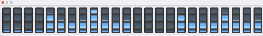
Rather unexpectedly the time taken using cpu for the initial tests was much less than using gpu (mps). I did wonder if I’d got the data switched, but repeating and checking cpu usage as shown below.

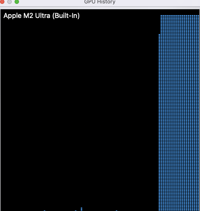
In contrast when using mps the gpu usage shot up

However for the larger data sets the times became comparable and around 7500 records the time taken is the same. Whilst inference is not as demanding as building the model it is not clear why cpu is better for the smaller data sets than gpu. As data sets get larger it might be expected that parallelisation on gpu might be advantageous, but I’ll investigate this in a subsequent post.

I also had a look at the performance on a M1 MacBook Pro Max, it was a little slower but still useful.